Piping
- Filip Hulsbosch
- Dennis De Beuckeleer
- Jonas Cleiren (Unlicensed)
- Kristof Smits
Drawing pipes
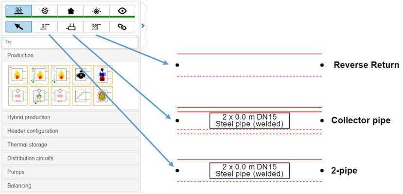
In Hysopt there are three different pipe types in heating as well as cooling. The selection of the pipes diameter is explained in the following chapter "Select pipes".
With the following token (ODI2fE9HdHRaRTRL) you see an example on how to draw a reverse return circuit in Hysopt.
Pipe parameters
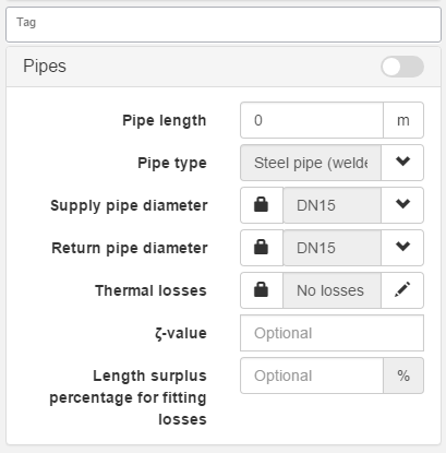
Follewing figure shows the parameter list on a pipe segment in Hysopt. Every pipe type has the same list of parameters.
The selection of the pipes diameter is explained in the following chapter of this Wiki "Select pipes". Pipe length and pipe type are self-evident.
Thermal losses
The thermal losses can also be added to the pipes. If you click on the pencil on the right in the main parameter list, the pop-up shown below will appear. The classes that can be selected are based on the German standard DIN EN 12828.
The isolation value changes depending on the pipe diameter, this is shown in the table below for class 1 to class 6. The thermal losses will be calculated during a dynamic simulation in function of the pipe length, pipe diameter, isolation class en the environment temperature.
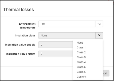
It is also possible to add a custom isolation. To do so, the user will need to fill in isolation value per diameter per pipe segment in Hysopt.
But this is a very time consuming job, therefore we advice to use the isolation classes.
Class 1 | Class 2 | Class 3 | Class 4 | Class 5 | Class 6 | Custom | ||
DN15 | 0,279 | 0,247 | 0,216 | 0,187 | 0,1598 | 0,1344 | 0,063 | W/mK |
DN20 | 0,293 | 0,257 | 0,224 | 0,193 | 0,1642 | 0,1346 | 0,069 | W/mK |
DN25 | 0,312 | 0,277 | 0,236 | 0,202 | 0,1708 | 0,1424 | 0,077 | W/mK |
DN32 | 0,332 | 0,288 | 0,248 | 0,211 | 0,1774 | 0,1472 | 0,085 | W/mK |
DN40 | 0,352 | 0,304 | 0,26 | 0,22 | 0,184 | 0,152 | 0,092 | W/mK |
DN50 | 0,392 | 0,335 | 0,284 | 0,238 | 0,1972 | 0,1616 | 0,107 | W/mK |
DN65 | 0,451 | 0,382 | 0,32 | 0,265 | 0,217 | 0,176 | 0,127 | W/mK |
Example parameters for the custom isolation in the table above
Lamda isolation = 0,021 W/mK
Isolation thickness = 0,06 m
Zeta- value
In addition to the linear pressure drops in the straight pipe pieces, additional pressure drops occur in the tubing network as a result of the resistance to the flow of water during changes in flow direction and / or water velocity. This occurs mainly at:
- bends, diameter transitions and taps in the distribution grid
- fittings such as collectors and closing, mixing or control cranes
- Devices like heaters, boilers, filters, batteries, heat exchangers etc.
The size of these local pressure losses can only be determined experimentally and is budgeted by a dimensionless local pressure-loss coefficient ζ.
If the ζ value is known, the pressure loss due to the local resistance can be calculated using the following formula:
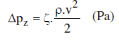
Wherein:
- DeltaPz: local pressure loss (in Pa)
- ζ: the local pressure loss coefficient
- rho: the volume of water (in kg / m³)
- v: speed of water (in m / s).
The user only needs to fill in the ζ-values for supply tube, Hysopt then calculates the additional pressure drop for the supply and return pipe.
In de following links can find some tables with ζ-values
.PNG?version=1&modificationDate=1492772890749&cacheVersion=1&api=v2)
.PNG?version=1&modificationDate=1492773140744&cacheVersion=1&api=v2)
Length surplus percentage
Instead of filling in all the ζ-values per pipe segment in Hysopt. The user can also choose to add a percentage extra pressure drop per pipe segment.
Depending on the tubing configuration of the installation, this percentage may vary from 10% to 40%, only when using steel pipes. With a normal configuration a percentage of 20% can be held. In case of an installation with many turns per meter, 30-40% can be held. When using a plastic tube, the percentage ranges from 50% to 70%, again depending on the tubing configuration
Selecting pipes in Hysopt
After the action "compute design flows" you go to the next step "Select pipes"
See Select pipes for more information