Real Time Simulation (RTS) versus Imposed Load Simulation (ILS)
- Kristof Smits
- Dennis De Beuckeleer (Unlicensed)
- Jonas Cleiren (Unlicensed)
Real Time Simulation (RTS)
When you design a hydraulic system in the 'traditional' Hysopt way, it will consist of one or more production units, pumps, distribution circuits and one or more zones.
Roomcontrollers, control logic and control valves are added to control the complete system.
During simulation the Hysopt software will calculate the 'real time' behaviour, as hydronic and thermodynamic time effects (like thermal inertia, cycle time of the control logic, ...) are applicable.
That’s why we call this method Real Time Simulation or RTS.
You can simulate with small or large horizons to assess control stability, hydraulic balance, hydraulic interactivity, comfort, temperature lack & excess in individual zones, etc.
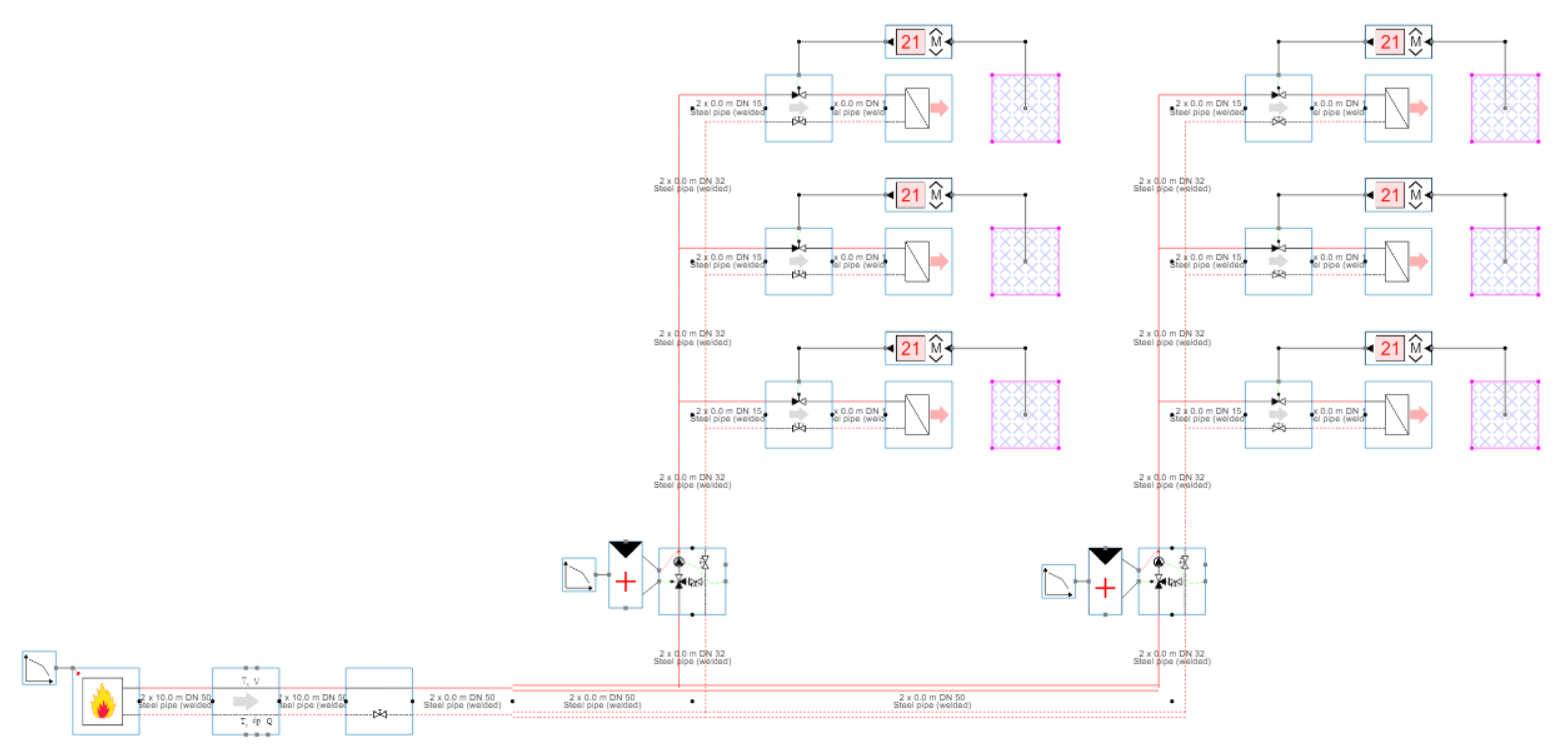
This figure [1] is an example of a RTS model of an apartment with 6 dwellings.
Advantages of RTS
Simulates the behaviour including real time behaviour like thermal inertia, control logic tability etc.
Suitable to assess control stability, hydraulic balance, hydraulic interactivity, comfort, individual HIU performance, temperature lack & excess in individual zones
Drawbacks of RTS
Time consuming to design large scale buildings and networks, like city districts with large appartment buildings
Simulation of large buildings and networks can be time consuming
- A small stepsize during simulation is necessary
Imposed Load Simulation (ILS)
A District Heating plant designer often wants to focus on the plant room and does not want to go in too much detail on the secondary side of the plant room.
In some cases detailed information about the secondary side is lacking, making it unuseful to engineer the secondary side in too much detail.
To resolve the drawbacks of RTS, and to support the DH plant designer, Hysopt created the 'Imposed Load Simulation' method (ILS) and the corresponding ILS building blocks.
The ILS building blocks are designed to reduce the level of detail of the so called secondary side of the plant room. .
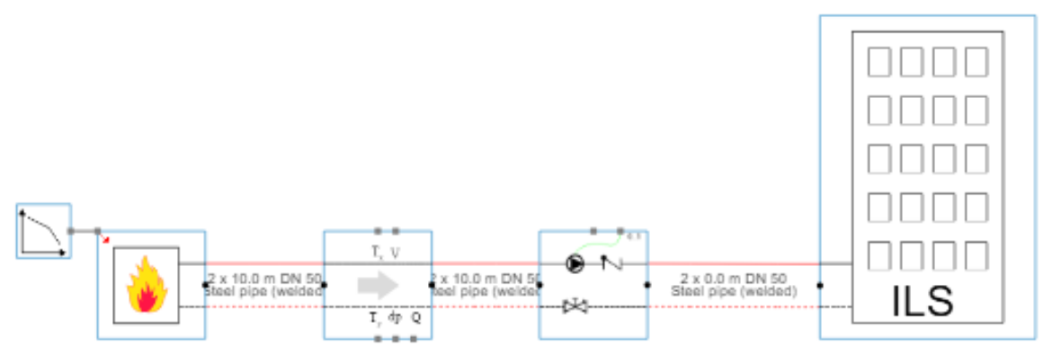
The model in figure [1] represents the exact same building as in figure [2]. As you can see the model is much more compact and scalable towards multiple buildings & dwellings.
No / less control logic
Another important difference between figure [1] (RTS) and figure [2] (ILS), is the visible control logic.
No room controllers, no control logic and no control valves are present.
This is typical for the ILS simulation technique : NO control logic needs to be added in the model to control the system.
Instead, the ILS building blocks will take care of the ‘control’ and will impose a certain load on the system.
In a nutshell, the ILS simulation technique works as follows.
Assumptions
In ILS mode, the software will make 3 important assumptions.
- ASSUMPTION 1 : The software assumes that the temperature in a dwelling is equal to its setpoint (day or night, dependent on the time), so implicitely it assumes that no comfort issues are applicable
ASSUMPTION 2 : The software assumes that that the heat demand in a dwelling is equal to the heat loss
ASSUMPTION 3 : the software assumes that each dwelling has the same type of radiators, same type of HIU’s, the same thermal losses and the same averaged daytime or nighttime temperature
- ASSUMPTION 4 : the software assumes that the system is balanced (during design of the system)
This actually means that the software neglects thermal inertia and assumes stable control logic, a hydraulic balanced system and no temperature lacks & excesses.
For the purpose of ILS, these are acceptable assumptions leading to a good approximation of heat loads and mass flows.
Simulation steps
During simulation, the software will execute following steps in each timestep for each ILS building block :
STEP 1 : the software calculates the thermal losses in each dwelling
STEP 2 : the software calculates the numbers of dwellings in tapping mode, in daytime heating mode and in nighttime heating mode
STEP 3 : a heat load generator calculates for each dwelling the heat demand (based on the heat loss and setpoints), and the resulting massflow & return temperature of the water
STEP 4 : The software will make sure that the design flows for Domestic Hot Water (DHW) and for Central Heating (CH) are never exceeded.
DHW : The diversity factor / flow as selected in the settings page will never be exceeded (directly in front of the building).
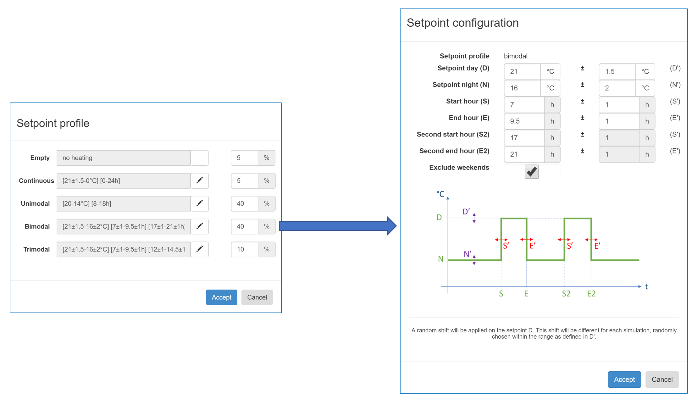
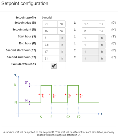
CH: The user is responsible to create a heating setpoint distribution for the ILS building (using the the setpoint configuration, as shown in figure [3])
in such a way that it matches the diversity factor central heating as selected in the settings page.
If there is a mismatch, the software will cap the flow and make sure the design flow is not exceeded, and a warming is displayed on the ILS block (see paragraph "ILS errors and common mistakes")For more information about diversity for DHW and CH, see [TODO]
- STEP 5 : if comfort problems are detected for more than 5% of the time, a warning is shown on the ILS building blocks.
This might indicate bad plant design or supply temperatures being too low. See the paragraph 'ILS errors' for more information - STEP 6 : the calculated massflows and return temperatures of all flats (in CH or DHW mode) are accumulated,
and ‘impose’ these onto the pipe primary to the building.
Advantages
- Reduces level of detail of the secondary side of the plant room
- Excellent to design, simulate and analyse plant rooms for district heating
- Very fast simulation speed
- Allows larger stepsizes if desired (only if not combined with RTS)
Drawbacks
- Some assumptions are made, resulting in an approximation and not all timing effects are taken into account
- Therefor not suitable to assess control stability, hydraulic balance (*), hydraulic interactivity, comfort, individual HIU performance, temperature lack & excess
- Requires some attention and knowledge on how to use ILS blocks (see the paragraph ILS errors and common mistakes)
(*) During simulation the flows are imposed by the ILS solver, so it is not possible to investigate hydraulic inbalance during simulation.
However during design calculation and optimisation of components, the actual flow rates (as displayed on the pipes) are calculated using RTS,
making it possible to investigate hydraulic balance during design, as you see in following example.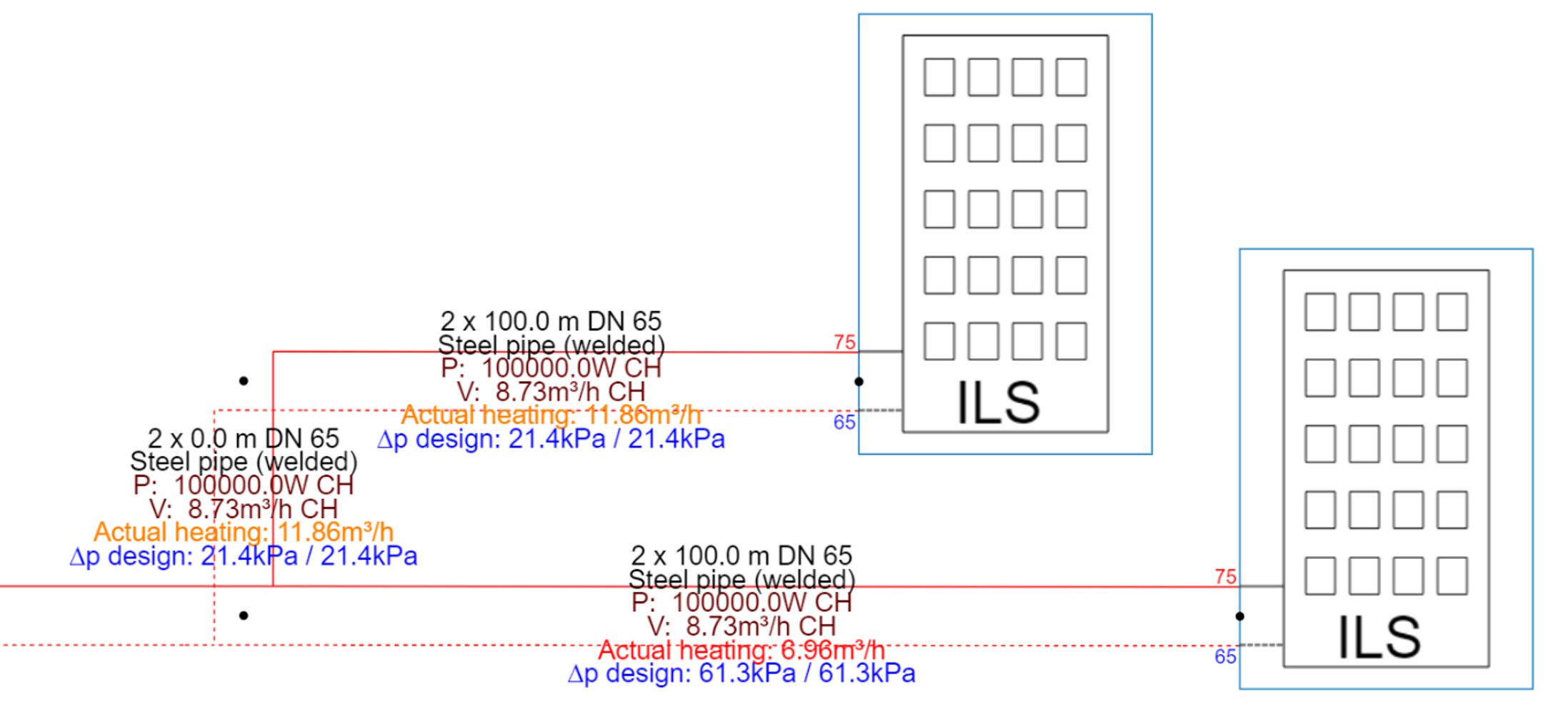
RTS combined with ILS
RTS and ILS design and simulation technique are compatible and can be combined within one hydraulic system,
as long as the RTS and ILS part are hydraulicly separated (e.g using a heat exchanger, an open header, a passive mixing circuit, ...).
An example of this combination is present in figure [4].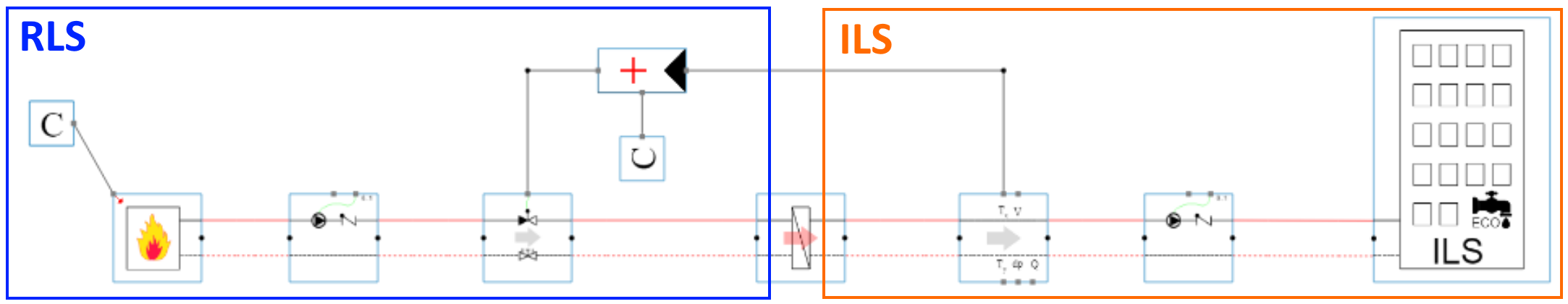
- In the left part (RTS) the flows are a result of the pump settings and the control valve positions
- In the right part (ILS) the flows are a result of the flows imposed by the ILS building blocks
In the ILS part it’s important that no control valves and/or control logic is added that interferes with the imposed flows (see paragraph "ILS errors and common mistakes")
ILS: errors and common mistakes
See Imposed Load Simulation (ILS) error codes and common mistakes
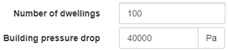
ILS input data
The first input data is the number of dwellings and the overall building pressure drop.
Direct heating
For direct heating the following information is needed to design the network:
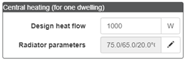
To correctly simulate the central heating, the user can specify the oversized ratio of the radiators or other end-users, the setpoint configurations and if needed enable or disable the heating. To get these input parameters, the simulation icon has to be clicked on.
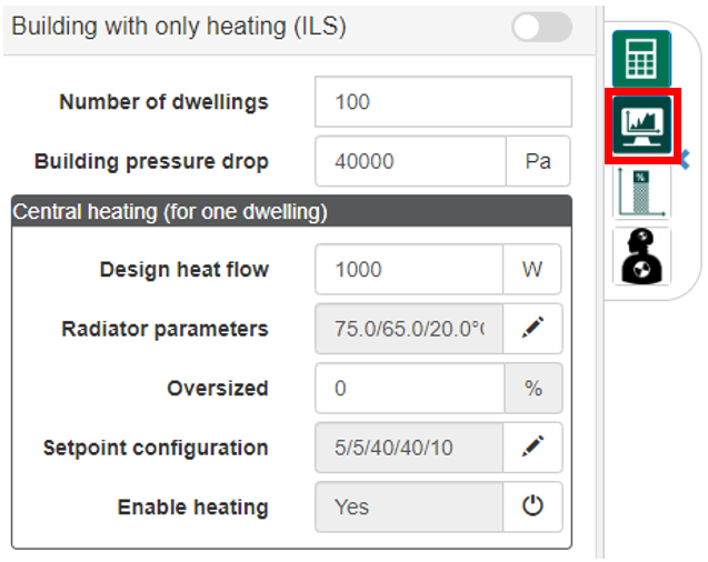
The setpoint configuration is done by clicking on the pencil icon and inserting the percentage of empty dwellings, dwellings with continuous, unimodal, bimodal and trimodal setpoints.
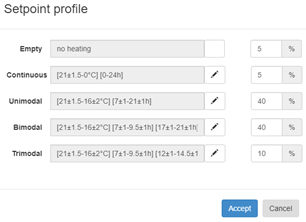
Further configuration is possible by clicking on the individual pencil icons and specifying the high and low setpoint, the start and end hour of every setpoint, and the randomness on time and temperature.
Indirect heating
Under construction
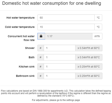
Domestic hot water (DHW)
For DHW the following information is needed to design the network:
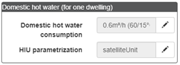
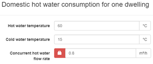
The default domestic hot water consumption for one dwelling can be altered by clicking on the pencil icon. The user can manually input the concurrent hot water flow rate for one dwelling, or unlocking it and specifying the amount and types of tapping points based on the DIN 1988-300 standard for apartments.
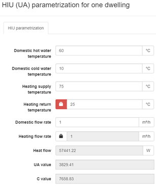
By clicking on the pencil next to the HIU parametrization, the user can specify the design conditions of the HIU. The manufacturers never give the required UA-value of the heat exchangers, although they do give the information needed to calculate the UA-value. (See Satellite units and simultaneous flows for more information about the calculation and parameterization of the HIU)
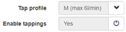
If the simulation icon is clicked on (see paragraph “Direct heating”), the user can specify the tap profile based on the Eco-design patterns, and if needed enable or disable the tappings.
ILS based on measurement data
Under construction
Timing examples
Under construction
Related pages
Floor plan implementation (for city plans)
Diversity and Aggregation (under construction)